Simple Linear Regression
OK, lets load the R mtcars data set, have a look at it and fit a simple linear regression model to a couple of the variables.
// Change directory to the one where the mtcars.csv file lives.
cd C:\Users\mjones\Dropbox\code-examples\stata\regression101
// Load csv
insheet using "mtcars.csv", clear
// Add a record ID
gen case_id = _n

// Descriptive stats and conditional listings of data
describe
list in 1/5
list  mpg cyl disp  hp drat  in 1/3
codebook mpg cyl
summarize mpg
summarize mpg, detail
tabulate carb gear
list car mpg if carb < 4

// Scatterplot matrix
graph matrix mpg cyl disp hp, half

// Basic regression
regress mpg hp
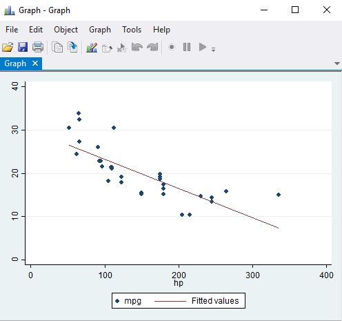
The results suggest that there is an association between miles per gallon and horse power. Specifically, for every unit increase in hp the mpg reduces by about 0.07 mpg.
We can use the model to make predictions for mpg and then plot them. You can also plot the residuals.
// Predict fitted values
predict fv
predict e, residual
twoway (scatter mpg hp) (lfit mpg hp)
Other items that can be generated from the model include:
| Description | Option for predict |
|---|---|
| residuals | resid |
| standardized residuals | rstandard |
| studentized or jackknifed residuals | rstudent |
| leverage | lev or hat |
| standard error of the residual | stdr |
| Cook’s D | cooksd |
| standard error of predicted individual y | stdf |
| standard error of predicted mean y | stdp |
Multiple Linear Regression
Now we fit a multivariate model and see that both number of cylinders and car weight are associated with mpg. Specifically, for each additional cylinder we see a 1.5 mpg reduction in the miles per gallon (holding weight constant). Similarly, for each 1000 lb increase in weight, the miles per gallon goes down by about 3.2 (holding the number of cylinders in the car constant). If we want to get an idea of the relative strength of the covariates (i.e. figure out what is explaining the majority of the variance) then we can issue the regress command with an added beta. Finally, we can treat the cylinder covariate as a factor by writing it with a i. prefix. This permits a non-linear relationship between the cylinders and mpg.
regress mpg cyl wt
regress mpg cyl wt, beta
regress mpg i.cyl wt

// Output from last command
------------------------------------------------------------------------------
         mpg |      Coef.   Std. Err.      t    P>|t|     [95% Conf. Interval]
-------------+----------------------------------------------------------------
         cyl |
          6  |  -4.255582   1.386073    -3.07   0.005    -7.094824    -1.41634
          8  |  -6.070859   1.652288    -3.67   0.001    -9.455418   -2.686301
             |
          wt |  -3.205614   .7538958    -4.25   0.000    -4.749899   -1.661328
       _cons |   33.99079   1.887794    18.01   0.000     30.12382    37.85776
------------------------------------------------------------------------------
Diagnostics
Inherent in using any statistical technique/model are simplifying assumptions and regression is no exception to this rule. The common diagnostic assessments include checking for:
- odd/influential data
- normality of residuals
- constant variance in the residuals
- multicollinearity
- linearity
- model specification
- independence of observations
- predictors are measured without error
Odd Looking Data
Data can look odd in a few ways, namely outliers, leverage and influence.
Outliers these are response values that are way out of the range of all the other response values. For example, maybe you have a persons height that has been entered as 180 metres instead of 1.8m. You can pick these up by reviewing the studentised resiudals.
// Outliers
predict r, rstudent
sort r
list sid state r in 1/10
list sid state r in -10/l
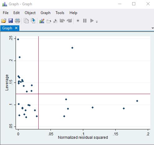
// Leverage
predict lev, leverage
stem lev
lvr2plot
// add , mlabel(var of interest) if you want to add a label to points
// Influence
predict d, cooksd
// Leave one out assessment
dfbeta
scatter _dfbeta_1 _dfbeta_2 _dfbeta_3 case_id, yline(.28 -.28)
Leverage relates to covariate values that are way beyond the rest of the covariate range. These kind of points can be highly influential on the parameter estimates.
Influential These are any points for that, if removed, would result in a big change in the parameter estimates. Cooks distance is a useful measure for global influential points. The higher the cooksd, the more influential - you are looking for points that are way outside the crowd rather than an absolute value. Another useful tool is the dfbeta. This indicates how much the parameter estimates change by leave-one-out analysis to assess the impact in terms of multiples of the parameter estimate standard errors.
So, if an observation has a dfbeta for the weight predictor of 0.29 then removing this point results increases the coefficient for weight by $0.29 \times se wt$. Typically any dfbeta in excess of $2/sqrt(n)$ merits investigation.
Added variable/Partial regression plots created with the avplot help you assess influential points. For example, the avplot for weight shows mpg and weight after adjusting for all other predictors. avplots produces these plots for all variables in one go.
If you identify potentially problematic points the thing to do first is assess the impact on the model parameters and prediction by fitting subsets of the data. In order to do this you can add a conditional statement at the end of the regress command.
Normality
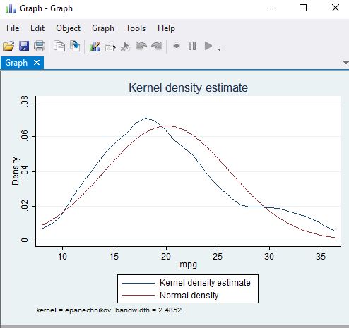
One of the assumptions for regression analysis is normality in the errors. The outcome (dependent) and predictor variables don’t need to be normally distributed. In fact, the residuals need to be normal only for the t-tests to be valid. So if you are interested in inference derived from the parameter t-tests then you need to concern yourself with normality.
Below is a kernel density estimate from the response and a qqplot of the residuals and a normal quantile plot graphs the quantiles of a variable against the quantiles of a normal (Gaussian) distribution.
We can also produce a normal probability plot since this kind of plot is sensitive to non-normality in the middle whereas qqnorm is more sensitive in the tails.
kdensity mpg, normal
qnorm r
pnorm r
| Distribution of mpg | QQplot |
|---|---|
 |
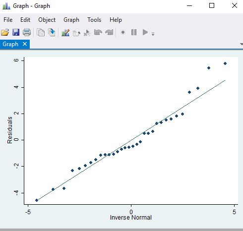 |
The above plots look OK as we do not see major deviations from normality. If we did see problems we might want to consider variable transforms such as log or square root on the covariates and/or response variable. Two commands that help with this are ladder and gladder.
ladder enroll
gladder enroll
Non-constant Variance
If you see non-constant variance in your residuals then your inference is likely to be incorrect. The easiest way to assess this is to simply look at the residuals against the fitted values. If you see a fan type pattern then you are in bother. There are various tests for non-constant variance, e.g. estat imtest and estat hettest but these are probably overkill.
rvfplot
Multicollinearity
If your covariates are correlated then it can lead to instability in the parameter estimates. A typical scenario where this comes up is when you have included both a term and squared version of the term in the same model. To assess use vif, ideally they should all be lower than 10. Centering variables can sometimes help if you seem to have a problem.
vif
Linearity
This is simply about ensuring you have a linear rather than curvilinear relationship between the response and the covariates.
Model Specification
This occurs when you have missed out an important variable from your model. The linktest is a good way to investigate this. linktest assumes that a regression is properly specified if one cannot find any additional independent variables that are significant except by chance. The _hat variable should be significant but the _hatsq should not be. ovtest is another command that is worth investigating.
Dependent Residuals
If you have clustering or repeat measures and you haven’t accounted for it in your model then you may have issues with the indepence assumption. To address this we can issue the cluster option in the regress command. We can test for independence using the Durbin Watson statistics - dwstat. Note that you have to issue tsset case_id first.