Statistical Rethinking is a great book for learning about Bayesian Modelling. In this first post of quite a few I am going to summarise some key points from the first three chapters, but mostly chapter 2 and 3. It is intended as a quick-ish reference so I will be skimming over a lot of content.
Table of Contents
I like examples so let’s dive in with the proportion of water covering the globe problem, hereafter the water/globe problem. In order to estimate this proportion we could take the globe throw it up in the air, catch it and record whether our index finger is on water or on land. If we do this enough times, we should be able to produce a reasonable estimate the proportion of water. Here is the data story is:
- The true proportion of water is $p$.
- A single toss has probability $p$ of our finger being on water and $1-p$ of being on land.
- We toss the globe the same way each time and all our tosses are independent of the others.
And assume we tossed the globe 9 times and for 6 of those tosses our finger lands on water. Now, Bayesian modelling takes prior knowledge and updates our understanding based on observed data. What is prior knowledge? It’s what you know before the first toss, e.g. that there is some water and some land so $p = 1$ is impossible. The appropriate lingua franca is that your posterior is proportional to the product of the likelihood and the prior. A few definitions:
Likelihood
This gives you information about the relative probability of any possible observation. The likelihood can be derived from the data story, here mapping to the binomial distribution. Specifically, we have the count of water observations $w$ is distributed binomially with probability $p$ over $n$ tosses of the globe.
$$ Pr(w|n, p) = \frac{n!}{w!(n-w)!}p^w (1-p)^{n-w} $$
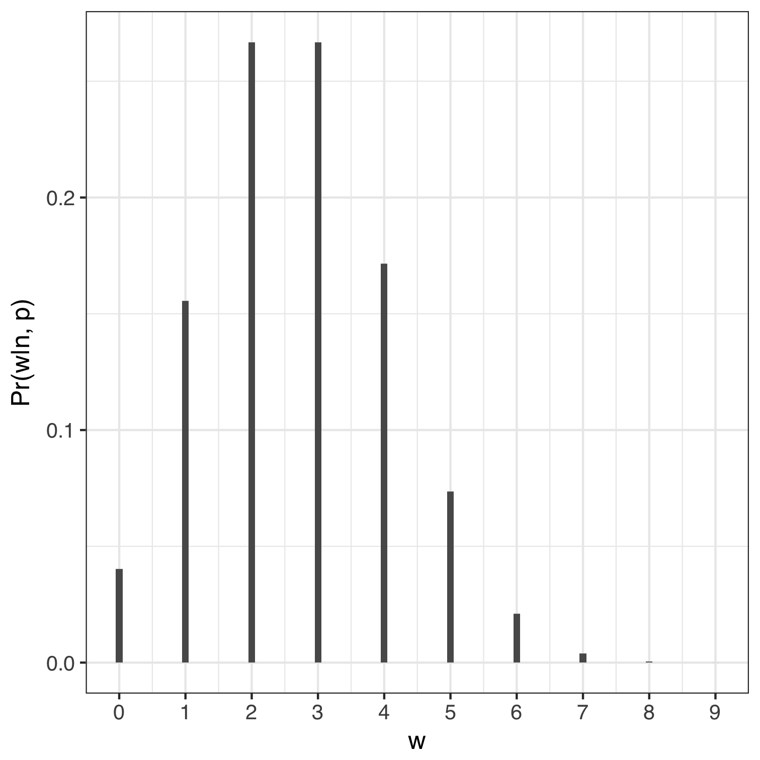
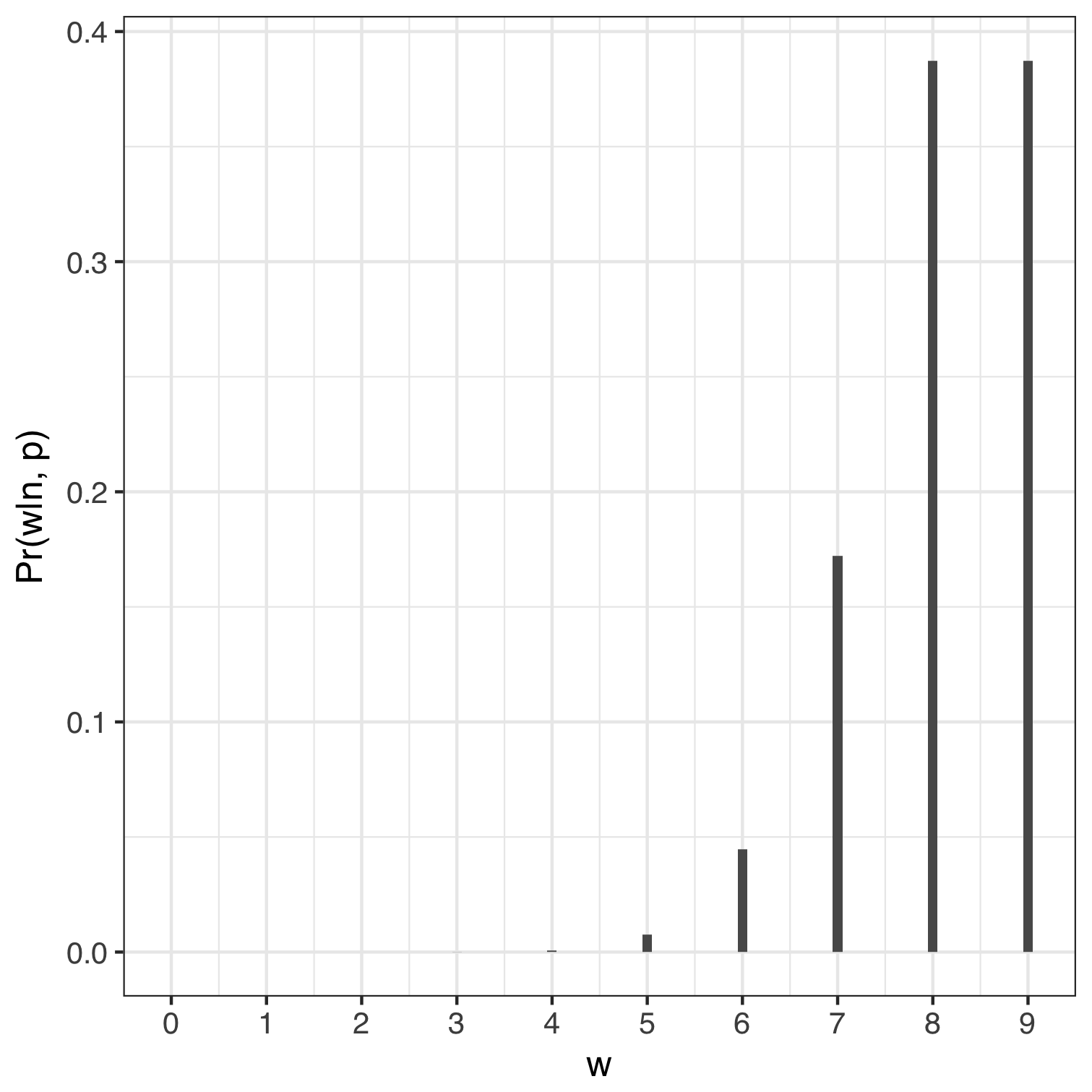
If we used a value of $p$ equal to 0.3 and 0.9 then the probability of us counting $0, 1, 2, .., 9$ instances of water can be computed in R using dbinom(0:9, size = 9, prob = 0.3) and are shown below. We can think of any of the bars representing the relative number of ways to get a specific number of $w$’s holding $n$ and $p$ constant. For example, the relative number of ways to get eight $w$’s is roughly zero when we assume $p = 0.3$ and about 40% when p = 0.9. In both cases the sum of the probabilities equals 1.
| Proportion of water = 0.3, n = 9 | Proportion of water = 0.9, n = 9 |
|---|---|
 |
 |
Parameters
In this case $p$ is our parameter of interest. Let’s move on.
Prior
The prior represents our initial view of the world – it is the initial probability that we assign to each possible value of $p$, which in this case ranges from 0 to 1. Priors can be uninformative, regularising or weakly informative and they help constrain parameters to plausible values, e.g. the proportion of water on the globe cannot be -10%. There will be more to say on this later.
Posterior
Once you have a likelihood, have identified the parameters you want to estimate together with a prior for each parameter we can obtain the posterior. This is a distribution which tells us the probability of the parameters conditional on the data and the model. Mathematically the posterior is proportional to the product of the likelihood and the prior. In order for the posterior to be a valid pdf, it needs to be normalised by dividing the product of the likelihood and prior by the average likelihood as follows:
$$ Pr(p|w) = \frac{Pr(w|p) \times Pr(p)}{Pr(w)} $$
$Pr(w)$ is commonly called the probability of the data, $Pr(w) = E(Pr(w|p))= \int Pr(w|p)Pr(p)dp$. These integrals get tough for any non-trivial case and so we use numerical methods such as grid approximation, quadratic approximation or Markov chain Monte Carlo. The simplest numerical approach for this example is to use the grid approximation.
A useful example for thinking about the normalising term is via the disease/test problem. The scenario states:
- there is a test that detects hiv 95% of the time; $Pr(+|hiv) = 0.95$
- the test gives false positives 1% of the time; $Pr(+|not \ hiv) = 0.01$, and
- hiv is relatively rare, say 0.1% of the population; $Pr(hiv) = 0.001$
So, if you test positive for hiv, what is the probability that you have hiv? In brief, we want $Pr(hiv|+result)$. However, this probability is a function of the probility of the disease in the community $Pr(hiv)$ and the probability that you get a positive test result conditional on having the disease. Using Bayes rule:
$$ Pr(hiv|+) = \frac{Pr(+|hiv) Pr(hiv)}{Pr(+)} $$
The denominator term is again the normalising constant and in this example can be computed by decomposition:
$$ Pr(+) = Pr(+|hiv)Pr(hiv) + Pr(+|not \ hiv)(1 - Pr(hiv)) $$
Which works through to about an 8.7% probability of actually having hiv.
Grid Approximation
Here is the process:
- Define a grid covering the parameters values.
- Compute the value of the prior at each value on the grid.
- Compute the likelihood at each parameter value.
- Compute the unstandardised posterior at each parameter value in the grid by multiplying the likelihood and prior.
- Standardise the posterior by dividing each value by the sum of the unstandardised posterior.
If our data comprised 9 tosses from which water fell under our finger in 6 times then here is how you use the grid approximation to compute and plot the posterior. The mode of the posterior suggests a central value for $p$ equal to $0.67$.
n.grid <- 100
p.grid <- seq(0, 1, length.out = n.grid)
# Uniform non-informative prior

prior <- rep(1, n.grid)
w <- 6
n <- 9
likelihood <- dbinom(w, size = n, prob = p.grid)
posterior <- likelihood * prior
posterior <- posterior / sum(posterior)
plot(x = p.grid, y = posterior, type = "l",
            xlab = "Probability of Water", ylab = "Posterior Probability")
p.grid[posterior == max(posterior)]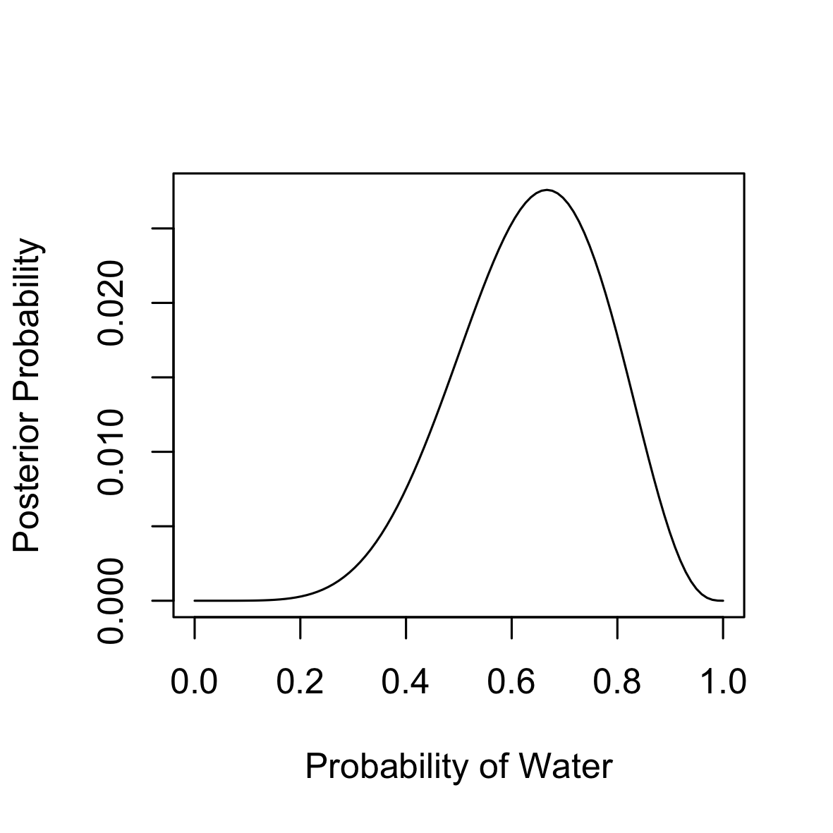
Quadratic Approximation
Quadratic approximation leverages the fact that the region near the peak of the posterior distribution will be normal-ish. So, this approach finds the posterior mode then computes the curvature near the peak which can be used to form the entire posterior distributions. The rethinking library has the map function to fit models using quadratic approximation.
globe.qa <- rethinking::map(
  alist(
    w ~ dbinom(9, p),  # binomial like

    p ~ dunif(0, 1)    # uniform prior

  ),
  data = list(w = 6)
)
# Parameter estimates

precis(globe.qa)
Which gives the following, i.e. making the assumption that the posterior is approximately gaussian, it is maximised at $p = 0.67$ and has a standard deviation of 0.16.
  Mean StdDev 5.5% 94.5%
p 0.67   0.16 0.42  0.92
The actual posterior here is a Beta distribution, but the approximation is reasonable in this case. Nevertheless, we need to note that the sample size is small here and that we need to be careful with small n.
Sampling
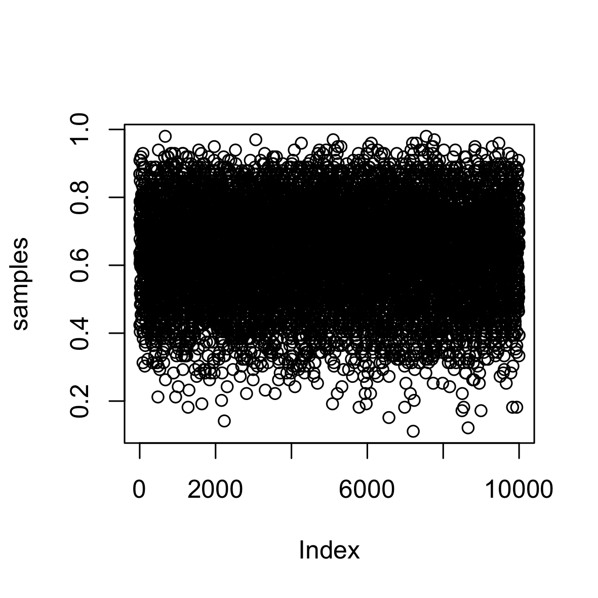
Generally, the end result of a Bayesian modelling exercise is a sample from the posterior distribution (unless you have a closed form solution). As such you need to work with the samples for conducting inference, but this isn’t such a bad thing. Earlier we obtained the posterior probability distribution from the water-globe problem and now the following should give you an idea of how to work with samples.
set.seed(4254)
samples <- sample(p.grid, prob = posterior, size = 1e4, replace = T)
plot(samples)
rethinking::dens(samples)| Sample | Density |
|---|---|
 |
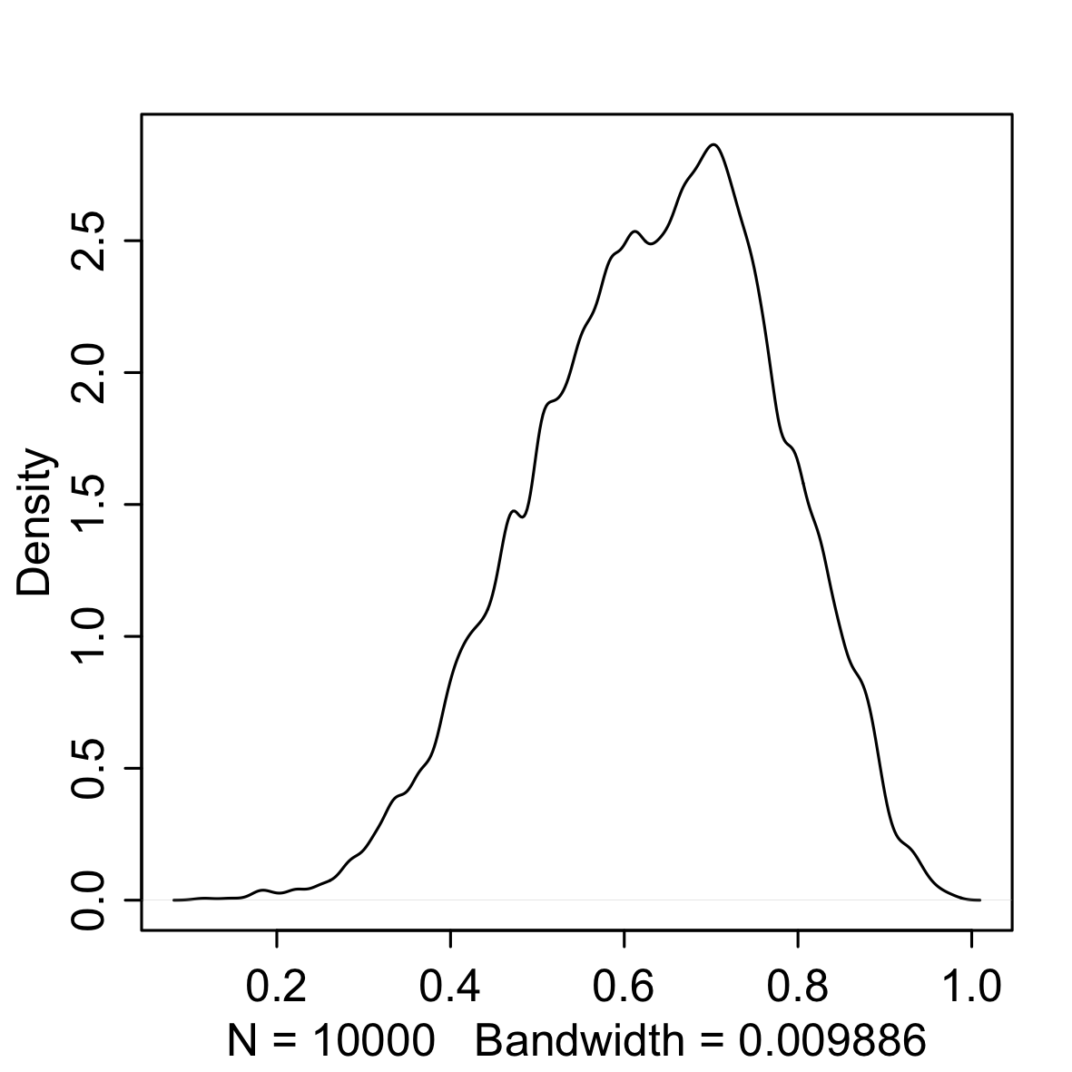 |
What we are doing is sampling from the original grid and we are telling sample to weight the possible values of the parameter based on the posterior probability. It is obvious that the density on the right is very similar to the distribution we got earlier simply by normalising the product of the likelihood and prior. However, we can now investigate our posterior distribution simply by referencing the sample. For example, we could:
- look at the probability that the parameter is less than 0.5,
- figure out what the parameter value of the lower 80% of the posterior
- form a credible interval or find the mode
- find the 60% highest posterior density interval for a skewed distribution (the narrowest interval that contains 60% of the distribution)
- compute point estimates
sum(samples < 0.5) / 1e4
quantile(samples, 0.8)
rethinking::PI(samples, prob = 0.95)
rethinking::HPDI(samples, prob = 0.95)
median(samples)
Loss Functions
A principled way to choose a point estimate is to make use of a loss function, which tells you the cost associated with using a particular point estimate. In the water/globe problem, say there is a real life proportion of water covering the globe. Now, I tell you a point estimate from the posterior and will $100 if I am right but will lose money proportional to the distance I am from the true value. Under this loss function I will minimise my losses by using the median. There will be more on loss functions in later posts.
Sampling to Simulate
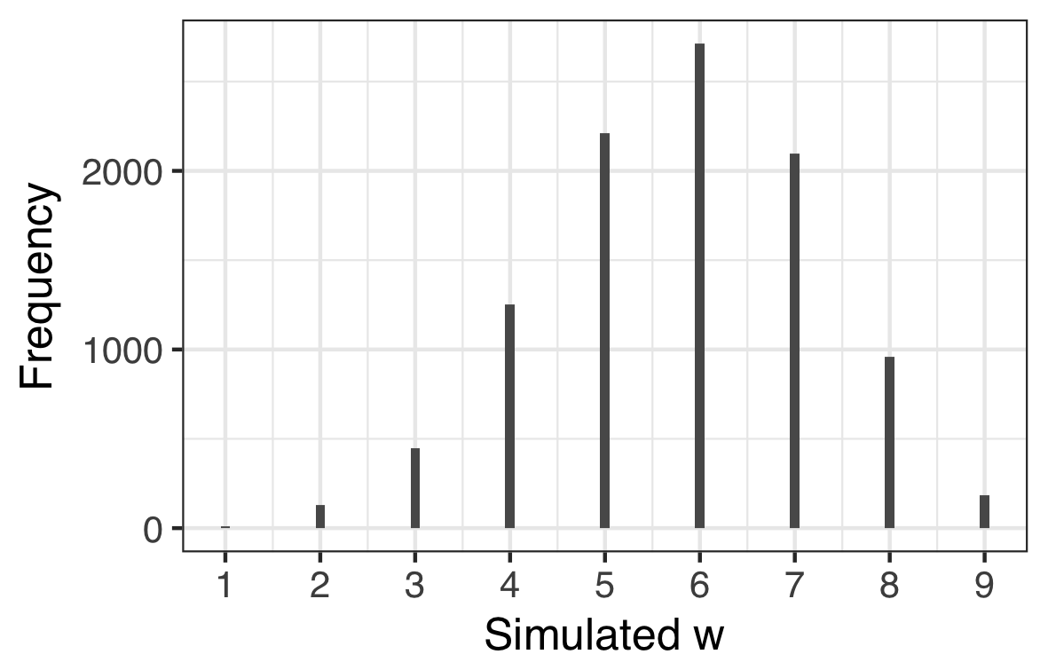
Bayesian models are generative. We obtained the posterior probability of our parameter (proportion of water on the globe) and we can use that distribution to simulate data via the binomial distribution we saw earlier:
$$ Pr(w|n, p) = \frac{n!}{w!(n-w)!}p^w (1-p)^{n-w} $$
For example, from the samples, the median estimate for $p$ is $p = 0.646$ so we can generate a large number of simulated observations by using our $n = 9$ and $p = 0.646$.
set.seed(3411)
sim1 <- rbinom(1e4, size = 9, prob = 0.646)
df <- data.frame(sim = sim1)
ggplot(df, aes(x = sim))+
  geom_bar(width = 0.1 )+
  scale_x_continuous("Simulated w", breaks = 0:9)+
scale_y_continuous("Pr(w|n, p)")| Simulation based on single $p$ | Posterior Predictive builds in uncertainty in $p$ |
|---|---|
 |
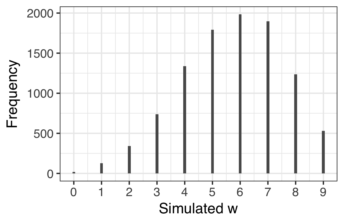 |
However, what we really would like to know is what the simulated data look like if we build in our uncertainty of the parameter estimate. When we do this we obtain a posterior predictive distribution. The way to do this is to use the samples as weights when simulating the data and this only necessitates a small tweak on the above code. The result is shown on the right hand side plot above. You can see how there is a much broader spread in $w$ reflecting our uncertainty about $p$.
set.seed(3411)
# Note that the number of simulated w's equals the

# number of samples but that isn't actually necessary.

sim1 <- rbinom(1e4, size = 9, prob = samples)
df <- data.frame(sim = sim1)
ggplot(df, aes(x = sim))+
  geom_bar(width = 0.1 )+
  scale_x_continuous("Simulated w", breaks = 0:9)+
  scale_y_continuous("Pr(w|n, p)")
In this case the posterior predictive distribution is quite consistent with the data we observed in that the distribution is centred around 6. We could assess the model in other ways for example assessing the longest run or the number of switches from water to land. The bayesplot package is quite a good way to explore these other options.