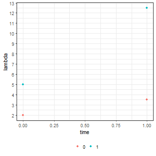
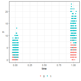
The following code constructs a hypothetical dataset describing the count of events observed in two groups (0 = control, 1 = treatment) at two times (0 = baseline, 1 = follow up) with means defined through a pre-specified model.
set.seed(250)

# Define the parameters

b0 <- 2
b1 <- 3
b2 <- 1.5
b3 <- 6

n <- 800
grp <- c(rep(0, n/2), rep(1, n/2))
time <- c(rep(0, n/4), rep(1, n/4), rep(0, n/4), rep(1, n/4))
# Model for the means

lambda <- b0 + b1 * grp + b2 * time + b3 * grp * time

df.fig <- data.frame(grp = grp, time = time, lambda = lambda)
# Generate poisson counts based on our means

df.fig$y <- rpois(n, lambda)

# The means

ggplot(df.fig, aes(x = time, y = lambda, colour = factor(grp))) +
  geom_jitter(height = 0, width = 0.05)

# The observed data

ggplot(df.fig, aes(x = time, y = y, colour = factor(grp))) +
  geom_jitter(height = 0, width = 0.05)
The means and simulated data are below:
| Means (lambda parameter) | Simulated data |
|---|---|
 |
 |
Now we fit a poisson regression model to the simulated data using the following commands:
summary(lm1 <- glm(y ~ grp * time, data = df.fig, family = poisson()))
exp(coef(lm1))

predict(lm1, type = "response", newdata = data.frame(grp = c(0, 0, 1, 1),
                                                     time = c(0, 1, 0, 1)))
which gives us parameter estimates and predicted values as follows:
Coefficients:
            Estimate Std. Error z value Pr(>|z|)
(Intercept)  0.67039    0.05057  13.256  < 2e-16 ***
grp          0.94404    0.05960  15.839  < 2e-16 ***
time         0.56071    0.06338   8.846  < 2e-16 ***
grp:time     0.38325    0.07348   5.216 1.83e-07 ***

exp(coef(lm1))
(Intercept)         grp        time    grp:time
   1.955000    2.570332    1.751918    1.467049

predict(lm1, type = "response", newdata = data.frame(grp = c(0, 0, 1, 1), time = c(0, 1, 0, 1)))
     1      2      3      4
 1.955  3.425  5.025 12.915
The exponentiated intercept, group and time parameters align with what we expect based on the model we specified. However, the interaction term is 1.50 which clearly does not equal 6. What is going on? The answer, in a word, is that the exponentiated parameter estimates are interpreted multiplicatively. We can find the correct interpretation through some simple calculations.
At baseline the model indicates that we expect to see $exp(0.67) = 1.96$ events in the control cohort whereas we expect to see $exp(0.67)exp(0.94) = 5.0$ events in the treatment cohort. Both these values are close to the means we specified, namely 2 and 5.
Similarly, at follow up the fitted value for the control group is $exp(0.67)exp(0.56) = 3.4$. Now, if the treatment were no different from the control intervention then we would expect to see something like $exp(0.67)exp(0.94)exp(0.56) = 8.80$ events at follow up. But this isn’t the case – the model says we expect to see $8.76 \times exp(0.38) = 12.92$ events. Thus, the exponentiated grp:time parameter suggests that we expect to see a $exp(0.38) = 1.47$ (or approx. 150%) increase ABOVE the change observed in the control group at follow up. Additionally, it is also worth to note that the interpretation is in terms of what we think the means look like there is no direct link back to our pre-specified parameters. If you do want to sanity check and recover estimates of the original parameters then you can specify the identity link as follows:
summary(lm1 <- glm(y ~ grp * time, data = df.fig, family = poisson(link = "identity")))Coefficients:
Estimate Std. Error z value Pr(>|z|)
(Intercept) 1.95500 0.09887 19.774 <2e-16 ***
grp 3.07000 0.18682 16.433 <2e-16 ***
time 1.47000 0.16401 8.963 <2e-16 ***
grp:time 6.42000 0.34147 18.801 <2e-16 ***