If you have multiple treatment options that lead to different outcomes, you will only be able to detect a difference in the average outcome under conditions where there is sufficient statistical power to do so. Statistical power is the probability that we detect an effect when there really is an effect to be detected. As statistical power increases the probability of making a Type II error (concluding there is no effect when, in fact, there is one) decreases.
Statistical power is affected by the size of the effect, the statistical significance criteria (typically 0.05) and the size of the sample. It is possible to miss a real effect simply by not taking a large enough sample. Power analyses help us by allowing us to explore the experimental conditions for a range of sample sizes.
In this post we look at how power varies in a logistic regression setting. First we compare treatment groups directly and then we compare treatment groups stratified by a characteristic of the mother that is also associated with the response of interest - e.g. a genetic disposition for a disease.
RCT Steroidal Treatments for Reducing the Risk of having an Ashthmatic Child.
Consider a steroidal intervention that influences the likelihood of having an ashmatic child. Assume a pilot study suggests the observed proportion of asthmatic kids in the control arm is 17.4% and in the treatment arm is 10%. This implies a relative risk (RR) of 0.575 - the probability of a kid having ashmatic in the treatment arm is 0.58 times that in the control arm.
Robert Grant gives us a way to convert odds-ratios (OR) to RR here, specifically $RR = \frac{OR}{1 – p + (p \times OR)}$. Turning this formula around we find the unadjusted odds-ratio is about 0.5329 - the odds of an “average” parent having an asthmatic kid in the treatment arm are around 0.53 times the odds of an equivalent parent having an asthmatic kid in the control arm.
Let’s say we want to work out a sample size for a formal parallel arm RCT. We suspect that we will only be able to get 650 people and the odds of an event in the intervention group are about half the odds of an event in the control group. What sort of power do we expect to obtain with this sample?
Method
Assume:
- Balanced groups (randomly selected) of 325 mothers per arm
- Proportion having asthmatic kid in control is 0.174
- The odds ratio associated with the steroidal treatment is 0.5329
- Adopt a linear predictor solely based on group membership
- Simulate a sample of kids by:
- Computing probability of asthma based on the exponentiated logits.
- Draw from binomial distribution parameterised as $Bin(n, p)$ where n is the (total) sample size and p the probability of ashmatic child.
- Fit a GLM with specification y ~ grp using the sample data and from this predict the probability for the control and treatment groups along with the difference in probability and estimated OR
- Bootstrap (299 replicates) to get the 0.025 and 0.975 quantiles of the difference
- Repeat the above 999 times
The above can be decomposed into separate functions - one to generate a simulated dataset, one to retrieve the bootstrap statistics of interest and one to contain these two, which we will call from a loop with 999 iterations.
Data Generation
This first function creates a dataset representative of the data we might observe in our real experiment. Each time the method is called a new data set will be created. Ignore the single nucleotide polymorphisms (SNP) variables for now.
get.data <- function(n.arm = 325,
                     p.ctl = 0.174,
                     or.trt = 0.5329,
                     or.snp = 1.5,
                     include.snp = F){

  # We create a linear predictor from which we generate data.

  # y ~ b0 + b1 * grp

  # or

  # y ~ b0 + b1 * grp + b2 * snp

  # The response of interest is asthma, denoted as 1/0 (yes/no).

  # Assume proportion in the ctl group with asthma is 0.174.

  # So, assuming the control group is the referant,

  # the baseline odds are:

  # p / (1-p) = 0.210653753

  # Taking the log of this gives us the intercept term

  # log(0.21) = -1.55754

  # The OR for intervention is 0.5329:

  # log(0.5329) = -0.6294215


  # Baseline odds:

  b0 <- log(p.ctl / (1 - p.ctl))
  # b1 is the coef for trt effect

  b1 = log(or.trt)

  # Group membership (0 = ctl, 1 = trt arm)

  grp <- c(rep(0, n.arm), rep(1, n.arm))

  snp <- NA

  if (include.snp){
    b2 = log(or.snp)

    # Genetic disposition to asthmatic kids in 86% of the population.

    # The 86% is arbitrary and made up just for the example.

    snp <- rbinom(n=2*n.arm, 1, prob = 0.86)

    # Linear predictor a combination of group and genetic disposition

    # for having an asthmatic kid

    logit.y <- b0 + b1 * grp + b2 * snp
  } else {
    # Linear predictor for the simple group comparison

    logit.y <- b0 + b1 * grp
  }

  # Gives us a randomly generated sequence of asthmatic kids

  # based on individual probability of event.

  p.y <- exp(logit.y)/(1 + exp(logit.y))
  y <- rbinom(n=2*n.arm, 1, prob = p.y)

  # Our pseudo sample.

  df.dat <- data.frame(id = 1:length(grp),
                       grp = grp,
                       snp = snp,
                       p.y = p.y,
                       y = y)

  return(df.dat)
}
Bootstrap Function
This function is used by the call to the boot function - more context can be found in the R help section for boot. Given a dataset and indices the function fits a GLM using a supplied formula/specification and returns estimates and predictions from the fitted model.
# Boot strapped logistic giving diff between proportions

boot.glm <- function(df.b,
                     indices,
                     myformula = myformula,
                     df.new = df.new) {

  # GLM Logistic

  d <- df.b[indices, ]
  m <- glm(myformula, family=binomial, data = d)

  prop <- predict(m, newdata = df.new, type = "response")
  p.ctl <- prop[1]
  p.trt <- prop[2]
  p.diff <- p.ctl - p.trt
  est.or <- exp(coef(m))[2]

  # s <- summary(m)

  # est.or.pval <- s$coefficients["stageint.2", "Pr(>|z|)"]


  as.numeric(c(p.ctl = p.ctl,
               p.trt = p.trt,
               p.diff = p.diff,
               est.or = est.or))
}
Simulation Function
This function encapsulates the code required to perform a single iteration of the simulation. It calls on the get.data described earlier then bootstraps a GLM model (with a pre-specified formula) to obtain parameter estimates and confidence intervals and dumps them into a data.frame that is returned to the calling function.
sim.glm <- function(x,
                    n.arm = 325,
                    p.ctl = 0.174,
                    or.trt = 0.5329,
                    or.snp = 1.5,
                    boot.reps = 299,
                    include.snp = F){


  df.dat <- get.data(n.arm = n.arm,
                     p.ctl = p.ctl,
                     or.trt = or.trt,
                     or.snp = or.snp,
                     include.snp = include.snp)


  # Specify the required formula to fit

  if(include.snp){
    myformula = y ~ grp + snp
    df.new <- data.frame(grp = c(0, 1), snp = 1)
  }else{
    myformula = y ~ grp
    df.new <- data.frame(grp = c(0, 1))
  }

  # Bootstrap

  bb <- boot::boot(df.dat,
                   statistic=boot.glm,
                   R=boot.reps,
                   myformula = myformula,
                   df.new = df.new)


  # First look at differences

  glm.prob.diff.est <- mean(bb$t[,3])
  glm.prob.diff.lwr <- as.numeric(quantile(bb$t[,3], probs = 0.025))
  glm.prob.diff.upr <- as.numeric(quantile(bb$t[,3], probs = 0.975))
  glm.prob.sig.diff <- ifelse(glm.prob.diff.est > 0 & glm.prob.diff.lwr > 0, 1, 0)

  # Now look at OR

  glm.or.est <- mean(bb$t[,4])


  # Note that for the snp tests, the probability of having an asthmatic kid

  # is conditional on presence of snp.

  if(include.snp){
    # names(df.dat)

    df.tmp <- df.dat[df.dat$grp==0 & df.dat$snp==0, ]
    n.pre <- nrow(df.tmp)
    p.pre <- sum(df.tmp$y)/nrow(df.tmp)

    df.tmp <- df.dat[df.dat$grp==1 & df.dat$snp==0, ]
    n.post <- nrow(df.tmp)
    p.post <- sum(df.tmp$y)/nrow(df.tmp)
  }else{
    n.pre <- nrow(df.dat)
    p.pre <- sum(df.dat$y)/nrow(df.dat)

    n.post <- nrow(df.dat)
    p.post <- sum(df.dat$y)/nrow(df.dat)
  }


  df.simres <- data.frame(n.pre = n.pre,
                          n.post = n.post,
                          p.pre = p.pre,
                          p.post = p.post,
                          glm.prob.diff.est = glm.prob.diff.est,
                          glm.prob.diff.lwr = glm.prob.diff.lwr,
                          glm.prob.diff.upr = glm.prob.diff.upr,
                          glm.prob.sig.diff = glm.prob.sig.diff,
                          glm.or.est = glm.or.est,
                          simid = x)

  df.simres
}
Bringing it together
Here we incorporate the functions into a monte carlo simulation. We initialise variables and then start a loop using parallel processing (to reduce run time if multiple cores are available). The results from each simulation is stored in the df.out2 data.frame. We can interogate df.out2 to get insight into the distribution of various estimates of interest.
# Initialise variables

set.seed(354)
nsim <- 999
n.arm <- 650/2 # c(500, 550, 600, 650, 700)

p.ctl = 0.174
or.trt = 0.5329
or.snp = 1.5
boot.reps = 299
include.snp = F

# Run the analysis in parallel across multiple CPU cores

# Initiate cluster

no_cores <- detectCores() - 1
cl <- makeCluster(no_cores)

# Specify all the functions that are required by the sim.

clusterExport(cl=cl, list("get.data", "boot.glm"))

l.res2 <- parLapply(cl,
                    seq(nsim),
                    fun = sim.glm,
                    n.arm = n.arm,
                    p.ctl = p.ctl,
                    or.trt = or.trt,
                    or.snp = or.snp,
                    boot.reps = boot.reps,
                    include.snp = include.snp)

stopCluster(cl)


df.out2 <- as.data.frame(do.call(rbind, l.res2))
mean(df.out2$glm.prob.sig.diff)
By setting the include.snp variable to TRUE we can run a second analysis using the same code that introduces a SNP covariate into the data generation process and the GLM specification to see what effect it has on power.
Results
The figure below shows the probability density for the lower bound of the difference in proportions of children born with asthma in each group. The central values for each group were 0.1 and 0.174 for the treatment and control groups respectively, aligning with the prespecified values. The proportion of the simulations where the lower bound of a 95% confidence interval for each of the estimated differences is greater than zero is 0.76, i.e. a little under 80%.
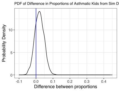
Important Note: We are looking at the difference in predicted proportions with asthma. We would get a different result if we were just looking at the significance of the odds ratio estimated from the GLM.
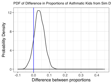
The next figure shows the same plot obtained from the analysis stratified by the SNP status. In this case the proportion of the simulations where the lower bound of a 95% confidence interval for each of the estimated differences is greater than zero is 0.87 giving 87% power.
Conclusion
By introducing a patient characteristic that was related to the response we were able to increase power without adjusting the sample size assumptions.