Imagine you are in the perilous and life threatening situation of being asked to generate random numbers. Compounding the peril is that we have also been asked to ensure that the probability of choosing a given number is linearly proportional to its magnitude.
OK, let’s start by imagining what the probability density function will look like - probably something list this:
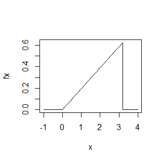
The area under the pdf must integrate to 1 so if the pdf is a linearly increasing function with support (arbitrarily say) 0 to 3.2 then the maximum density of the above must be equal to 0.625. This comes from the formula for the area of a triangle $\frac{1}{2}base \times height$.
$$
\frac{3.2 \times h}{2} = 1 \\
=> h = 0.625
$$
And so the gradient of our wedge equals $m = 0.625 / 3.2 \approx 0.195$ and can define the pdf as:
$$f_x(x) = \left\{\begin{array} {ll} 0.195 x & 0 \le x \le 3.2 \\\ 0 & otherwise \end{array}\right. $$
You can check if you like but the above integrates to 1. We want to generate values that are distributed according to $f_x(x)$ and cumulative probability distribution $F_x(x)$. The trick to doing this is to note that if $y = F_x(x)$ has a uniform distribution on $[0, 1]$ then $F_x^{-1}(y)$ has the same distribution as $x$.
The integral of $f_x$ is (obviously) just $\frac{0.195x^2}{2}$ and the inverse of this function is:
$$ F_x^{-1}(x) = \sqrt{\frac{2x}{0.195}} $$
because
$$ F_x^{-1}(F(x)) = \sqrt{\frac{2 \times \frac{0.195x^2}{2}}{0.195}} = x $$
Aside - the way you work out the inverse function is to put $z = \frac{0.195x^2}{2}$ then replace the $z$ with $x$ and $x$ with $z$ and then solve for $z$.
OK, all we have to do now is generate $u$ from a standard uniform distribution, compute x such that $F_x(x) = u$ and then take x to be the random number from our wedgy distribution. The code for this is as follows:
# Work out maximum density
h <- 1/((1/2) * 3.2)
# m is the slope of the pdf
m <- h / 3.2
# so the following is the pdf for 0 to 3.2
x <- seq(0, 3.2, by = 0.2)
fx <- m * x
plot(x, fx, type = "l")
# Now apply the inverse cdf method:
# generate standard uniform
u <- runif(1000)
# throw the u random variable into the inverse cdf
x <- sqrt(2 * u / m)
# x should be distribution as per fx
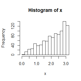
hist(x)Which gives the following histogram and that’s close enough to the target distribution for me!