The title was stolen directly from the excellent 2016 paper by Tanner Sorensen and Shravan Vasishth. Here I recreate their analysis using brms R package, primarily as a self-teach exercise. I am going to very much assume that the basic ideas of Bayesian analysis are already understood. I will add some informtion on prior and posterior predictive checks because I think not doing so missing a large part of the point of a Bayesian analysis. The original tutorial provided a hands-on introduction to fitting LMMs in a Bayesian framework using the probabilistic programming language Stan.
Let’s start with the data. In brief the we have reading times (rt) in milliseconds of the head noun of the relative clause recorded in two conditions with 37 subjects and 15 items. The data have some missing values, but the focus here was on a complete case analysis because missing values are a can of worms in Stan and deserve a tutorial of their own. In total we are looking at 547 data points.
Quoting Sorensen:
A subject relative is a sentence like “The senator who interrogated the journalist resigned” where a noun (senator) is modified by a relative clause (who interrogated the journalist), and the modified noun is the grammatical subject of the relative clause. In an object relative, the noun modified by the relative clause is the grammatical object of the relative clause like “The senator who the journalist interrogated resigned”. In both cases, the noun that is modified (senator) is called the head noun.
You can pick up what you need here and save it to a local folder, but you can also read that file directly. We only need a part of the data so lets wrap it up in a function.
library(tidyverse)
library(brms)

get.data <- function(){
  df.r <- read.table('https://raw.githubusercontent.com/vasishth/BayesLMMTutorial/master/data/gibsonwu2012data.txt')
  # head(df.r)


  df.r <- df.r %>%
    dplyr::filter(region == "headnoun") %>%
    dplyr::select(-word) %>%
    dplyr::mutate(subj = as.factor(subj),
                  item = as.factor(item),
                  so = ifelse(type == "subj-ext", -1, 1))
  # head(df.r)

  # sort(as.numeric(unique(df.r$subj)))

  # sort(as.numeric(unique(df.r$item)))

  # nrow(df.r)


  return(df.r)
}


df.r <- get.data()

# Distribution of reading times.

plot(density(df.r$rt), main = "Distribution of reading times")
In the above code you will note that the so variable contains an indicator of ‘o’ (object relative) and ’s’ (subject relative) that are coded as 1 and -1 respectively. When coding up Stan models you need to be a bit more careful with your data – we might come back to this later.
The brms package supports a wide range of (non-)linear multivariate multilevel models using Stan for full Bayesian inference. Many distributional assumptions are supported. Additionally, brms provides the capability of extracting the underlying Stan code and thus gives a useful starting point if you want to do something more complicated. As a starting point we ignore the (very likely) possibility of correlated measures and fit a fixed effect model. We use weakly informative priors, but not the current stan-dev reccommendations nor a Cauchy1 distribution as per Gelman et al. 2008 paper. Here, we adopt Normal priors, simply because they are easy to think about and rationalise. For reference, the parameterisations of the brms supported distributions can be found here.
An Initial Model
Prior to looking at the data, what do we know about average reading speed? Well, obviously, the lower bound is a little be greater than zero and a high value might be a couple of seconds. So, lets just say a typcial value is about 1000 millisecs and you could expect anywhere between about 100 and 2000 milliseconds and that gives us some guidance on what the intercept looks like. We are pulling numbers out of the air here, but at least we have a rough idea of what the typical value might be and we can (should) conduct sensitivity analyses with uninformative priors (that typically correspond with frequentist results).
$$ rt_i \sim Lognormal(\mu_i, \sigma) \\\ \mu_i = \beta_0 + \beta_1 so_i \\\ \beta_0 \sim Normal(6, 1) \\\ \beta_1 \sim Normal(0, 10) \\\ \sigma \sim Student-t(3, 0, 10) $$
OK, let’s fit a model. The brms package can have multi-dimensional formula so we specify the formula explicitly as myf and use this approach repeatedly.
# brms formula, more later...

myf <- bf(rt ~ so)
priors <- get_prior(myf,
                    data = df.r,
                    family = lognormal())
priors$prior[1:2] <- "normal(0, 10)"
priors$prior[3] <- "normal(6, 1)"
priors

blm0 <- brms::brm(myf,
            data = df.r,
            family = lognormal(),
            prior = priors,
            control = list(max_treedepth = 10),
            iter = 2000,
            chains = 2, cores = 6, seed = 5453, save_model = "brm1.txt")
summary(blm0, waic = TRUE)
The blm0 is an instance of a brmsfit object. The summary view gives the following output, which is similar to the fixed effects model presented by Sorensen. What are these results telling us? First, the Rhat values are equal to 1, so the chains look like they converged OK. Second, the reading time for subject-relative has a central value around $exp(6.06 + 0.04) = 446$ millisecs and the object-relative has a central value of around $exp(6.06 - 0.04) = 412$ millisecs. These values align to the exponentiated mean of the log reading times for the two groups.
 Family: lognormal
  Links: mu = identity; sigma = identity
Formula: rt ~ so
   Data: df.r (Number of observations: 547)
Samples: 2 chains, each with iter = 2000; warmup = 1000; thin = 1;
         total post-warmup samples = 2000
    ICs: LOO = NA; WAIC = 7625.74; R2 = NA

Population-Level Effects:
          Estimate Est.Error l-95% CI u-95% CI Eff.Sample Rhat
Intercept     6.06      0.03     6.01     6.11       1917 1.00
so           -0.04      0.03    -0.09     0.01       2000 1.00

Family Specific Parameters:
      Estimate Est.Error l-95% CI u-95% CI Eff.Sample Rhat
sigma     0.60      0.02     0.57     0.63       2000 1.00

Samples were drawn using sampling(NUTS). For each parameter, Eff.Sample
is a crude measure of effective sample size, and Rhat is the potential
scale reduction factor on split chains (at convergence, Rhat = 1).
The marginal posterior distributions for each of the three parameters are shown below. The distribution of b_s0 is mostly below zero suggesting that the object-relative is easier to read. However, the 95\% credible interval includes zero so the evidence is not particularly strong. Unlike frequentist analyses, the results give us a view on the uncertainty in the error term (sigma) which ranges from 0.57 to 0.63 on the log scale.
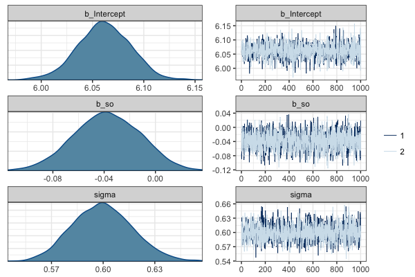
Posterior distribution for estimated parameters
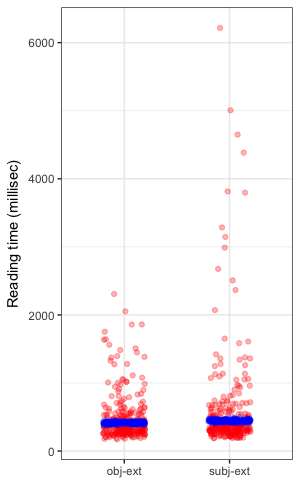
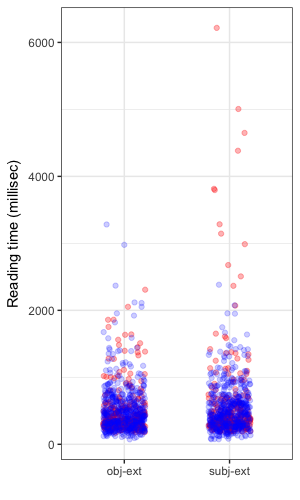
Here’s a view of the observed data overlayed with the posterior distribution for reading times showing the estimated typical reading time. The right hand plot shows a posterior predictive distribution, which embodies both the uncertainty inherent in our distributional assumption for the response and the uncertainty in the estimated parameters. The idea behind examining the posterior predictive distribution is that it should generate data that looks similar to the observed data. McElreath provides the clearest exposition I have read on this concept. The posterior predictive is a simulation of our original data conditional on the observed values.
| Posterior means | Posterior predictive |
|---|---|
 |
 |
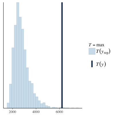
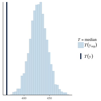
Another option for model checking is to use the bayesplot package, which provides a swag-full of posterior predictive checks that are more sophisticated than the single generated dataset shown above. Below we can see that simulated data has a much lower maximum value than that observed in the original data and the median of the simulated values is actually quite a lot higher than we observed. Both these diagnostics suggest the current model does not characterise the data well.
| PPC (max) | PPC (median) |
|---|---|
 |
 |
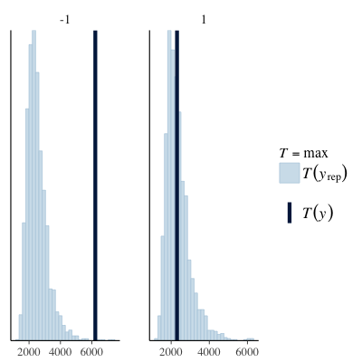
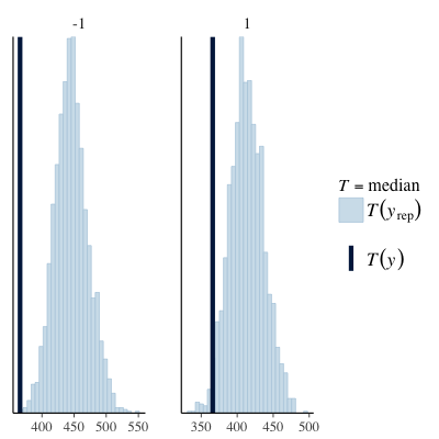
Posterior predictive checks grouped by subject and object relative (see below) appear to show that the issues manifest to a greater extent in the subject relative group. An outline of the code for the last few plots is also shown below.
| PPC (max) | PPC (median) |
|---|---|
 |
 |
# Look at the posterior distribution

m.post <- as.matrix(blm0)
nrow(m.post)
df.post1 <- data_frame(type = c(rep('subj-ext', 2000), rep('obj-ext', 2000)),
                      rt = c(m.post[,1] - m.post[,2], m.post[,1] + m.post[,2])  )
set.seed(324)
idx <- base::sample(1:nrow(df.post1), 600, replace = F)
df.post1 <- df.post1[idx, ]

# Posterior

ggplot(data = df.r , aes(x = type, y = rt))+
  geom_jitter(width = 0.2, height = 0, colour = "red", alpha = 0.3)+
  geom_jitter(data = df.post1, aes(x = type, y = exp(rt) ),
              width = 0.2, height = 0, colour = "blue", alpha = 0.2)+
  ylab("Reading time (millisec)") + xlab("")


# Single draw just for demonstration

pp.tmp <- brms::posterior_predict(blm0, newdata = data.frame(so = c(-1, 1)))
dim(pp.tmp)

df.post2 <- data_frame(type = c(rep('subj-ext', 2000), rep('obj-ext', 2000)),
                      rt = c(pp.tmp[,1], pp.tmp[,2])  )
set.seed(284729)
idx <- base::sample(1:nrow(df.post2), 1000, replace = F)
df.post2 <- df.post2[idx, ]
str(df.post2)

ggplot(data = df.r , aes(x = type, y = rt))+
  geom_jitter(width = 0.2, height = 0, colour = "red", alpha = 0.3)+
  geom_jitter(data = df.post2, aes(x = type, y = rt ),
              width = 0.2, height = 0, colour = "blue", alpha = 0.2)+
  ylab("Reading time (millisec)") + xlab("")


# More useful PPC

library(bayesplot)
ppc_dens_overlay(df.r$rt, yrep[1:50, ])

ppc_stat(df.r$rt, yrep, stat = "max")
ppc_stat(df.r$rt, yrep, stat = "median")

ppc_stat_grouped(df.r$rt, yrep, stat = "max", group = df.r$so)
ppc_stat_grouped(df.r$rt, yrep, stat = "median", group = df.r$so)
Relaxing the equal variance assumption
While Sorensen do not explore this avenue, one possibility is that we may have reasonable distributional assumptions but the notion of a shared variance across groups may not be accurate. The brms package readily supports this refinement via its forumla interface that we used earlier. We do not nominate any priors for the sigma model parameters so they will just be assigned uninformative defaults.
myf <- bf(rt ~ so, sigma ~ so)
priors <- get_prior(myf,
                    data = df.r,
                    family = lognormal())
priors$prior[1:2] <- "normal(0, 10)"
priors$prior[3] <- "normal(6, 1)"

blm1 <- brm(myf,
            data = df.r,
            family = lognormal(),
            prior = priors,
            control = list(max_treedepth = 10),
            iter = 2000,
            chains = 2, cores = 6, seed = 5453, save_model = "brm1.txt")
summary(blm1, waic = TRUE)
The results (below) suggest that the variation in reading times are different across subject and object groups. However, posterior predictive checks on the maximum and median values (not shown) are still not representative of the observed values. We won’t take this further yet, but we might return to it later.
 Family: lognormal
  Links: mu = identity; sigma = log
Formula: rt ~ so
         sigma ~ so
   Data: df.r (Number of observations: 547)
Samples: 2 chains, each with iter = 2000; warmup = 1000; thin = 1;
         total post-warmup samples = 2000
    ICs: LOO = NA; WAIC = 7614.42; R2 = NA

Population-Level Effects:
                Estimate Est.Error l-95% CI u-95% CI Eff.Sample Rhat
Intercept           6.06      0.02     6.01     6.11       1897 1.00
sigma_Intercept    -0.53      0.03    -0.58    -0.46       2000 1.00
so                 -0.04      0.03    -0.09     0.01       1768 1.00
sigma_so           -0.11      0.03    -0.17    -0.05       1892 1.00
Modelling the Repeat Measures
Given we know there are repeat measures in the data, we should model it as such or risk violating an assumption of independence. We do this by specifying person-level and item-level variability in the model. I won’t say most, but a lot of people refer to these as random intercepts. Here is the revised model. You can see that the $\beta_{person[i]}$ and $\beta_{item[i]}$ make adjustments to the intercept term dependent on the particular person and the particular item, hence the random intercept terminology.
$$ rt_i \sim Lognormal(\mu_i, \sigma) \\\ \mu_i = \beta_0 + \beta_{person[i]} + \beta_{item[i]} + \beta_1 so_i \\\ \beta_0 \sim Normal(6, 1) \\\ \beta_{person} \sim Normal(0, \sigma_{person}) \\\ \beta_{item} \sim Normal(0, \sigma_{item}) \\\ \beta_1 \sim Normal(0, 10) \\\ \sigma, \sigma_{person} , \sigma_{item} \sim Student-t(3, 0, 10) $$
It is a straight forward exercise to ask brms to fit this model. For the sake of simplicity, we will not continue to model the standard deviation across groups and I haven’t specified all the priors but it would be simple to do so.
# Random effects model

df.r <- get.data()
myf <- bf(rt ~ so + (1|subj) + (1|item))
priors <- get_prior(myf,
                    data = df.r,
                    family = lognormal())
priors$prior[1:2] <- "normal(0, 10)"

# > priors

#                   prior     class      coef group resp dpar nlpar bound

# 1         normal(0, 10)         b

# 2         normal(0, 10)         b        so

# 3 student_t(3, 5.9, 10) Intercept

# 4   student_t(3, 0, 10)        sd

# 5                              sd            item

# 6                              sd Intercept  item

# 7                              sd            subj

# 8                              sd Intercept  subj

# 9   student_t(3, 0, 10)     sigma


blm2 <- brm(rt ~ so + (1|subj) + (1|item),
            data = df.r,
            family = lognormal(),
            prior = priors,
            control = list(max_treedepth = 10),
            iter = 2000,
            chains = 2, cores = 6, seed = 5453, save_model = "brm1.stan")
summary(blm2)


post1 <- brms::posterior_predict(blm2)
dim(post1)
head(post1[,1])
hist(post1[,1])
bayesplot::ppc_dens_overlay(df.r$rt, post1[1:50, ])
The results show us that the modelling the subject level and item level variance was worthwhile in that both the random intercept variance estimates are substantially above zero. Additionally, the estimates align closely with those of Sorensen. However, the estimate for the difference between the reading times continues to represent only weak evidence of an effect.
 Family: lognormal
  Links: mu = identity; sigma = identity
Formula: rt ~ so + (1 | subj) + (1 | item)
   Data: df.r (Number of observations: 547)
Samples: 2 chains, each with iter = 2000; warmup = 1000; thin = 1;
         total post-warmup samples = 2000
    ICs: LOO = NA; WAIC = NA; R2 = NA

Group-Level Effects:
~item (Number of levels: 15)
              Estimate Est.Error l-95% CI u-95% CI Eff.Sample Rhat
sd(Intercept)     0.20      0.05     0.12     0.32        655 1.00

~subj (Number of levels: 37)
              Estimate Est.Error l-95% CI u-95% CI Eff.Sample Rhat
sd(Intercept)     0.26      0.04     0.19     0.35        867 1.00

Population-Level Effects:
          Estimate Est.Error l-95% CI u-95% CI Eff.Sample Rhat
Intercept     6.06      0.07     5.92     6.21        588 1.01
so           -0.04      0.02    -0.08     0.01       2000 1.00

Family Specific Parameters:
      Estimate Est.Error l-95% CI u-95% CI Eff.Sample Rhat
sigma     0.52      0.02     0.49     0.55       2000 1.00
Next we introduce varying slopes into the model, which allows us to characterise the variation in the difference in reading time across individuals and items. As per Sorensen, we initially prohibit correlation between the varying interecpts and slopes. The required implementation is as follows.
df.r <- get.data()
# The latter (-1 + ) part prevents correlation between random effects

(priors <- get_prior(bf(rt ~ so +
                         (1|subj) + (-1 + so |subj) +
                         (1|item) + (-1 + so|item)),
                    data = df.r,
                    family = lognormal()))
priors$prior[1:2] <- "normal(0, 10)"
blm3 <- brm(rt ~ so +
              (1|subj) + (-1 + so |subj) +
              (1|item) + (-1 + so|item),
            data = df.r,
            family = lognormal(),
            prior = priors,
            control = list(max_treedepth = 10),
            iter = 2000,
            chains = 2, cores = 6, seed = 5453, save_model = "brm1.stan")
summary(blm3)
VarCorr(blm3)
While there is evidence for including the random slopes, the estimate of the difference between subject and object relatives has weakened.
Family: lognormal
  Links: mu = identity; sigma = identity
Formula: rt ~ so + (1 | subj) + (-1 + so | subj) + (1 | item) + (-1 + so | item)
   Data: df.r (Number of observations: 547)
Samples: 2 chains, each with iter = 2000; warmup = 1000; thin = 1;
         total post-warmup samples = 2000
    ICs: LOO = NA; WAIC = NA; R2 = NA

Group-Level Effects:
~item (Number of levels: 15)
              Estimate Est.Error l-95% CI u-95% CI Eff.Sample Rhat
sd(Intercept)     0.20      0.05     0.12     0.32        797 1.00
sd(so)            0.04      0.03     0.00     0.11        782 1.00

~subj (Number of levels: 37)
              Estimate Est.Error l-95% CI u-95% CI Eff.Sample Rhat
sd(Intercept)     0.25      0.04     0.18     0.34        668 1.01
sd(so)            0.06      0.03     0.00     0.13        619 1.00

Population-Level Effects:
          Estimate Est.Error l-95% CI u-95% CI Eff.Sample Rhat
Intercept     6.06      0.08     5.92     6.22        458 1.00
so           -0.04      0.03    -0.09     0.02       2000 1.00

Family Specific Parameters:
      Estimate Est.Error l-95% CI u-95% CI Eff.Sample Rhat
sigma     0.52      0.02     0.49     0.55       2000 1.00
Finally, we remove the restriction on correlation between the varying slopes and intercepts as implemented below.
df.r <- get.data()
(priors <- get_prior(bf(rt ~ so +
                          (1 + so|subj) +
                          (1 + so|item)),
                     data = df.r,
                     family = lognormal()))
priors$prior[1:2] <- "normal(0, 10)"
# mypriors1 <- c(brms::set_prior("cauchy(0, 2.5)", class = "b"))

blm4 <- brm(rt ~ so +
              (1 + so|subj) +
              (1 + so|item),
            data = df.r,
            family = lognormal(),
            prior = priors,
            control = list(max_treedepth = 10),
            iter = 2000,
            chains = 2, cores = 6, seed = 5453, save_model = "brm1.stan")
summary(blm4)
The results suggest no correlation between the varying intercepts and slopes for the item but a negative correlation between the person level varying intercepts and slopes. The implication is that if a person has a slower than average reading time then they will read object relatives.
 Family: lognormal
  Links: mu = identity; sigma = identity
Formula: rt ~ so + (1 + so | subj) + (1 + so | item)
   Data: df.r (Number of observations: 547)
Samples: 2 chains, each with iter = 2000; warmup = 1000; thin = 1;
         total post-warmup samples = 2000
    ICs: LOO = NA; WAIC = NA; R2 = NA

Group-Level Effects:
~item (Number of levels: 15)
                  Estimate Est.Error l-95% CI u-95% CI Eff.Sample Rhat
sd(Intercept)         0.21      0.05     0.13     0.33        660 1.00
sd(so)                0.04      0.03     0.00     0.10        961 1.00
cor(Intercept,so)    -0.00      0.53    -0.92     0.92       2000 1.00

~subj (Number of levels: 37)
                  Estimate Est.Error l-95% CI u-95% CI Eff.Sample Rhat
sd(Intercept)         0.25      0.04     0.19     0.34        624 1.00
sd(so)                0.07      0.03     0.01     0.13        680 1.00
cor(Intercept,so)    -0.61      0.30    -0.98     0.16       1392 1.00

Population-Level Effects:
          Estimate Est.Error l-95% CI u-95% CI Eff.Sample Rhat
Intercept     6.06      0.07     5.92     6.21        492 1.00
so           -0.03      0.03    -0.09     0.02       1160 1.00

Family Specific Parameters:
      Estimate Est.Error l-95% CI u-95% CI Eff.Sample Rhat
sigma     0.51      0.02     0.48     0.55       2000 1.00
Unfortunately, that is all I have time for today. Hopefully, I will get an opportunity not to far in the future to check the interpretation and add some more details.