I find the Statistical Rethinking text very helpful in conveying Bayesian concepts. Here I simply try to condense some of the introductory material. The text is supported with R and Python implementations and there is a youtube lecture series on which the text is based.
OK, Bayesian Analysis?
Let’s start with inference. What we are talking about here is about using the information available to you in order to arrive at rational conclusions that your mum still won’t have a bar of. Bayesian analysis is a fairly snappy way to go about this task.
Now, let’s get serious and work up to laying down some definitions and notation. First, the breed of inference we are interested in here is statistical inference. Statistical inference involves using observations in a framework of presupposition and statistical models that aim at a logical conclusions. Generally we want to be able to make some statements about a scientific question relating to a population of interest.
Examples - we flip a coin obtained from the local mint 10 times and it produces 7 heads. Should we believe the coin is fair? What about the other coins produced by the mint? We measure the heights of 10 men that play for a professional basket ball team. What does this tell us about the height of all men? Bayesian analysis gives us a formal method to combine what we already know with new evidence and characterises the remaining uncertainty in probability.
The Standard (Zombie) Example of Bayesian Inference
In a bayesian analysis we characterise uncertainty using a small bag of tools. Let’s introduce a few…
A Prior
The Bayesian framework places our existing knowledge in a probability distribution and a probability distribution simply captures how likely a variable of interest is across its possible range. For example, the proportion of zombies hanging around the local shopping mall must be somewhere between zero and 100%1 of all the individuals there. Now, perhaps we are sceptical, but not entirely calm, about the notion that zombies exist. So let’s start this off and believe that we believe that the most likely situation is that there are no-need-for-tears-at-bedtime zero zombies. However, because we subscribe to the philosophy of the belt and braces brigade, let’s assume that it could be the case that up to 30% of the individuals in the mall are of the zombie variety. If we had to draw a picture our relative belief we might produce something like this:
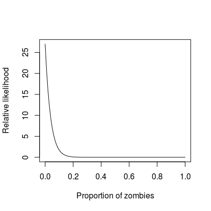
I generated that snappy curve from a Beta distribution by using paramter values equal to 1 and 27. In a more mathy bent we say:
$$ \theta \sim Beta(1, 27) $$
In words - theta is distributed as a random variable originated from a beta distribution with shape parameters 1 and 27 - you can see why we favour the mathy version.
Likelihood
Now, let’s go to the mall and pick out 20 people at random under the assumption that all individuals have the same probability of being a zombie. However, not one of the people in the sample tries to even take a nimble at us and so we conclude (with perhaps undue certainty) that the sample we picked contained no zombies. We can, again, make this more formal by saying that the data generating process was a Binomial distribution where one of the parameters is our sample size and the other parameter represents the probability that a randomly selected individual is a zombie. Mathematically, we have:
$$ y|\theta \sim Bin(20, \theta) $$
and therefore conditional on $\theta$ any given sample of mall people stands a chance of containing a zombie.
Posterior
In light of our sample data our state of belief has changed and we maybe feeling a bit better about going to the shops. Anyway, in the Bayesian world, a simple relationship allows us to characterise our new knowledge, again in terms of a probability distribution known as the posterior2. The relationship between the posterior, prior and likelihood is derived as a consequence of the laws of probability3 and has the form:
$$ Posterior = \frac{Likelihood \times Prior}{Average \ Likelihood} $$
The average likelihood bit is computed over all the possible values of the parameter $\theta$ - the proportion of zombies which must be somewhere between zero to 1. Fortunately, we don’t have to know how to work out the above directly because the product of a Beta prior and a Binomial likelihood is well known. Specifically, it is another Beta distribution but with different parameters based on the the data we observed and the prior parameters. The first parameter of the posterior beta distribution is $a + y$ and the second is $b + n - y$. In our case, a = 1, y = 0, b = 27 and n = 20 so we have the posterior is:
$$ Pr(\theta|y) \sim Beta(1, 47) $$
If we were to draw another graph of the (new) relative strength of beliefs it would look something like the following (new beliefs in red):
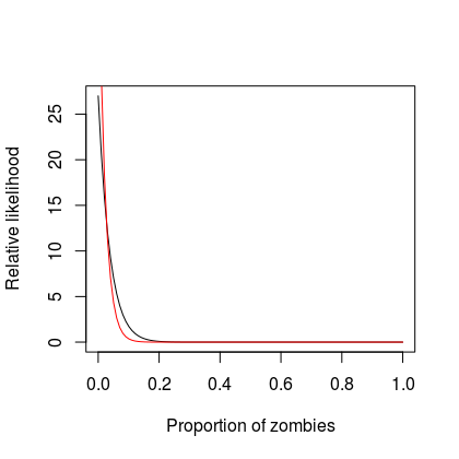
So whereas initially we were 90% certain that less than 8.5% of the population are zombies, now we are 90% certain that less than 5% of the population are zombies. We have reduced our uncertainty by leveraging our existing beliefs and our sample observations.
Grid Approximation
Unfortunately, the calculations are rarely this simple - we rarely have conjugate pairs of priors and likelihood like I contrived in the above example. However, we can get around this using sampling. In its simplest form we can use a grid approximation.
In R the following code shows how this might play out. We first set up a posterior distribution and then we sample with replacement to get an approximation of the posterior distribution.
# This is the range of parameter values and defines the precision
# to which we can estimate the parameter of interest.
mygrid <- seq(0, 1, length.out = 1000)
# Defines our prior beliefs
prior <- dbeta(mygrid, 1, 27)
# Defines the relative likelihood of the data (zero zombies out of 20)
# across all the possible parameter values
likelihood <- dbinom(0, size = 20, prob = mygrid)
# Compute the posterior and normalise it
posterior <- likelihood * prior
posterior <- posterior / sum(posterior)
# This is analytic posterior - generally we don't have the
# luxury of knowing this.
analyticpost <- dbeta(mygrid, 1, 47)
# Sample from the posterior distribution
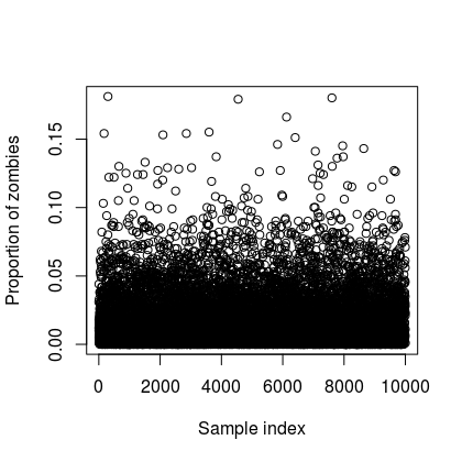
myposteriorsample <- sample(mygrid, prob = posterior, size = 1e4, replace = T)
# Plot the samples
plot(myposteriorsample, type = "p",
xlab = "Sample index",
ylab = "Proportion of zombies")
# Plot the analytical and the sampled posterior distribution
x.idx <- density(myposteriorsample)$x
y.den <- density(myposteriorsample)$y
plot(mygrid, analyticpost, type = "l",
xlab = "Proportion of zombies",
ylab = "Relative likelihood", xlim = c(0, 0.3))
lines(x.idx, y.den, col = "red")
| Samples from posterior | Analytic and sampled posterior (red) probability density |
|---|---|
 |
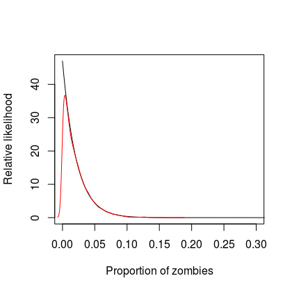 |
Clearly the relatively likelihood at approximately zero is underestimated by the sampling approach but this is to do with the available precision and could be improved by increasing the resolution of the grid.
The grid approximation is useful to get some understanding into the mechanics but does not scale well to more complex problems where we would more commonly use Markov Chain Monte Carlo MCMC simulations.
Posterior Summaries
It is interesting to consider (moreso if you are a bit nerdy) how you might summarise our new state of knowledge inherent in the posterior distribution. There are a few options to condense what it is telling us into a 10 second soundbite for people without patience or interest.
First, we can compute a 95% credible interval as below, which tells us that there is a 95% probability that the proportion of zombies in the community is between zero and 7.5%. A similar interval is the Highest Posterior Density Interval, but this interval is the narrowest interval that contains the specified probability mass. For this example it turns out to be about the same as the credible interval but that won’t always be the case. We can obtain the point estimates of the mean, median and mode, which turn out to be 2.1%, 1.4% and 0.37%.
All of these approaches are effectively data reduction techniques - we have reduced the posterior probability distribution to a one or two numbers in order to make what it is telling us more digestable.
# Credible interval
quantile(myposteriorsample, c(0.025, 0.975))
rethinking::PI(myposteriorsample, 0.95)

# HPDI
rethinking::HPDI(myposteriorsample, 0.975)

# Measures of centrality
mean(myposteriorsample)
median(myposteriorsample)

# Mode
rethinking::chainmode(myposteriorsample)
Another thing we can do is define a loss function and characterise the cost of adopting a particular summary under given conditions. This mostly comes into play when we want to make a decision such as whether we should go to the shops or not. Different loss functions imply different point estimates and a common loss function is to assume that the loss is proportional to the absolute difference between your decision and the correct answer. We can compute the loss over the entire parameter range using the following code, which gives us an value of 1.4%, identical to the median computed previous. In reality the loss function would need more thought and we might make the cost function penalise being wrong more harshly as might be well advised since encountering a zombie has stark metaphyscial implications.
loss <- sapply(mygrid, function(d) sum(analyticpost * abs(d - mygrid)))
mygrid[which.min(loss)]loss <- sapply()
Model Checking
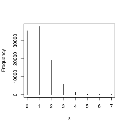
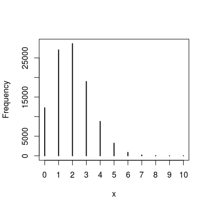
I know I have been banging for a bit now, but this last bit is important so stick with it. Here is the thing - all Bayesian models are generative so once you have a posterior distribution of the parameter of interest you can simulate new data. Ideally the predictions we make should contain both uncertainty in the distribution associated with a parameter and the uncertainty about the parameter itself. For example, if we use $\theta = 0.05$ or $\theta = 0.1$ we get a distribution of zombies like the figures below. So if there is a 5% probability that an individual is a zombie we would expect to zero or one zombies most of the time. However, if there was a 10% probability that an individual is a zombie we would mostly expect to see 1 or 2 in a sample of 20. In a nutshell, when $\theta = 0.05$ we expect to see a zero count of zombies more often than we do if $\theta = 0.1$.
| Proportion of zombies 5% | 10% |
|---|---|
 |
 |
Now, the thing is, $\theta$ also has uncertainty as we have described by the posterior distribution and ideally we want to propagate this uncertainty into our predictions. To do this we average all of the prediction distributions together using the posterior of each value of $\theta$. This gives us a posterior predictive distribution, which is actually a lot easier to produce than to explain, the following gets us to where we want to be.
# Distribution of observed zombies theta = 0.05
z1 <- rbinom(1e4, size = 20, prob = 0.05)
# Distribution of observed zombies averaged across the posterior distribution
z2 <- rbinom(1e4, size = 20, prob = myposteriorsample)
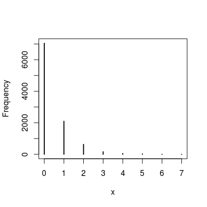
In this case we can be quite conforted by the fact that the posterior predictive aligns fairly well with what we observed since it looks like we generally encounter small numbers (0 or 1) zombies in our daily trip to the shops.